Monte CarloQuantitative FinancePythonTypeScript

Pricing an option three ways

Black–Scholes, Monte Carlo and finite-difference Greeks: three methods that should agree, and a playground to see what happens when the conditions change.

By Paolo Minhas•Independent learning project• View the code

Monte Carlo simulation is a standard tool in physics: Geant4, which I used for detector simulation on HIBEAM, is built on it. This project looks at the same idea from a different side, how it is used in finance to price and risk-manage derivatives.

Under the Black–Scholes model the price of a European option can be written down exactly, which makes it a good test bed: the closed form tells you whether a simulation is right. The playground below lets you change the conditions and watch the methods respond.

Try it

Black–Scholes price of the call

10.4506

These are the inputs behind the Python results table further down (S = K = 100, r = 5%, σ = 20%, T = 1 year). The closed-form numbers here should match it, and the Monte Carlo ones should agree within their standard errors.

value today payoff at expiry

Intrinsic value

0.0000

at the money right now

Time value

10.4506

100% of the price

Chance of finishing in the money

56.0%

under the model's risk-neutral measure

The grey line is what the option pays at expiry. The orange curve is what it is worth today: always above the payoff, because there is still time for the price to move. Shorten the expiry or lower the volatility and the curve collapses onto the payoff; lengthen it or raise the volatility and it lifts away.

How the three methods work

A call pays $\max(S_T - K,\,0)$ at expiry, where $S_T$ is the asset price then and $K$ is the strike (a put pays $\max(K - S_T,\,0)$ ). The model assumes the price follows geometric Brownian motion, and under the risk-neutral measure that has an exact solution:

S_T = S_0 \exp\!\Big(\big(r - q - \tfrac{1}{2}\sigma^2\big)T + \sigma\sqrt{T}\,Z\Big), \qquad Z \sim \mathcal{N}(0,1)

1. Black–Scholes closed form

Taking the discounted expected payoff exactly gives, for a call,

C = S_0 e^{-qT}\,\Phi(d_1) - K e^{-rT}\,\Phi(d_2), \qquad d_{1,2} = \frac{\ln(S_0/K) + \big(r - q \pm \tfrac{1}{2}\sigma^2\big)T}{\sigma\sqrt{T}}

with $\Phi$ the standard normal CDF. The Greeks (delta, gamma, vega, theta, rho) are its derivatives and have closed forms too. This is the benchmark.

2. Monte Carlo

Because $S_T$ is known exactly, no time-stepping is needed: draw $Z$ , form the payoff, average and discount.

V \approx \frac{e^{-rT}}{N}\sum_{i=1}^{N}\max\!\big(S_T^{(i)} - K,\,0\big), \qquad \mathrm{SE} = \frac{s}{\sqrt{N}}

The standard error SE ( $s$ is the sample standard deviation of the discounted payoffs) is what tells you how far to trust the answer, and it falls only as $1/\sqrt{N}$ . Antithetic variates pair each draw $Z$ with $-Z$ and average the pair: the two payoffs are negatively correlated, so the average is less noisy for the same number of paths.

3. Greeks by bumping

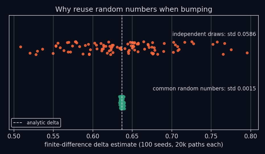
\frac{\partial V}{\partial S} \approx \frac{V(S+h) - V(S-h)}{2h}

With Monte Carlo prices this only works if both prices use the same random numbers. Otherwise each price carries independent noise, and dividing that noise by a small $h$ swamps the signal. Reusing the draws (common random numbers) makes the errors cancel. Gamma, a second difference, is the most sensitive to this.

Results from the Python library

The reference case is S = K = 100, r = 5%, σ = 20%, T = 1 year. The playground above is a TypeScript port of the same engine: its closed-form prices and Greeks agree with the Python values to about 10⁻¹⁵, which a script in the repository checks.

Method	Call	Put
Black–Scholes (closed form)	10.4506	5.5735
Monte Carlo, 1M paths	10.4276 ± 0.0147	5.5608 ± 0.0086
Monte Carlo, 1M paths, antithetic	10.4284 ± 0.0104	5.5576 ± 0.0066

The error shrinks as $1/\sqrt{N}$ , as it should, and antithetic variates cut the standard error by about 30% here at no extra cost per path.

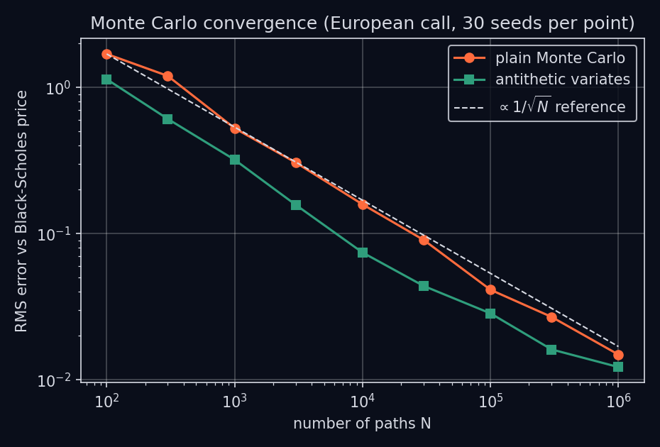
Log-log plot of Monte Carlo RMS error against number of paths, following a 1/√N line, with antithetic variates lower than plain Monte Carlo.

RMS error against the Black–Scholes price, 30 seeds per point.

Greek (call)	Analytic	Common random numbers	Independent draws
delta	0.6368	0.6368	0.6463
gamma	0.01876	0.01856	−0.03789
vega (per 1.00)	37.524	37.601	39.521

Bump-and-reprice with 400,000 paths. With independent draws the gamma comes out negative, which is impossible for a long option. Across 100 repeated runs, sharing the random numbers cut the spread of the delta estimate by roughly a factor of 40.

Strip plot of 100 delta estimates: widely scattered with independent draws, tightly clustered on the analytic value with common random numbers.

Limitations

Constant volatility (geometric Brownian motion), so no volatility smile or skew.
European exercise only: no early exercise and no path-dependent payoffs.
Gamma by bumping is noisy because the payoff has a kink. Pathwise or likelihood-ratio estimators are the usual fix.
A learning project, not a trading tool. It uses no market data and the numbers are not advice.

The code

The Python library has 20 tests: put–call parity, the Monte Carlo price landing within a few standard errors of Black–Scholes, the 1/√N scaling, and the bump-and-reprice Greeks against the analytic ones. The core of the Monte Carlo pricer:

The full library, tests and the script that regenerates these figures are on GitHub.